Origami Mathematics by Chris Ward

Below is a cut-down version of my Final Year Project from the University of Sussex where I studied Computer Science & Artificial Intelligence from 2001 to 2004. I have picked out the sections focused on the mathematics involved.

My 20-year-old self apologises for any mistakes. Actually, he's probably moved on by now.

The result of the maths was a paper-folding demo which I made for the project. Have a play!

Huzita's origami axioms

Huzita has formulated what is currently the most powerful known set of origami axioms:

Given two points p₁ and p₂ we can fold a line connecting them.
Given two points p₁ and p₂ we can fold p₁ onto p₂.
Given two lines l₁ and l₂ we can fold line l₁ onto l₂.
Given a point p₁ and a line l₁ we can make a fold perpendicular to l₁ passing through the point p₁.
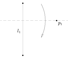
Given two points p₁ and p₂ and a line l₁ we can make a fold that places p₁ onto l₁ and passes through the point p₂.
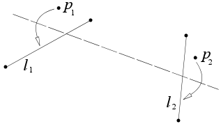
Given two points p₁ and p₂ and two lines l₁ and l₂ we can make a fold that places p₁ onto line l₁ and places p₂ onto line l₂.

Each Axiom provides a method for folding the fold-line. This is an extremely vital process of the system, as it enables various ways for users to create folds.

Only the first three Axioms may be necessary in Implementation, but the others can be used in possible extensions to the system.

Notion of 'Fold-points' and 'Fold-lines'

The following are ideas I have come up with, whilst analysing and thinking about origami modelling. The idea of 'fold-points' and 'fold-lines' are original (although similar ideas will obviously appear elsewhere).

When thinking about ways to make a fold, you need points and lines (see Axioms). But how do you get these points and lines?

When you have the initial unfolded rectangular paper, you have 4 edges and 4 corner points. These make up the possible fold-lines and fold-points.

Fold-lines are lines on the paper which can be folded along, or used to make other fold-lines (using the axioms). Fold-points are all the points which can be used in the axioms to create new fold-lines.

Each time a fold is made; more fold-points are created. These fold-points are essentially all the intersections between the fold-lines of a paper model.

Similarly, each time a fold is made; more fold-lines are created.

In Figure 1 we have four fold-points (1,2,3,4) and four edges (A,B,C,D) which can be used as fold-lines. After folding point 1 we have Figure 2. We have gained two more fold-points (5,6), changed one fold-point (1), and gained three edges (E,F,G) for possible fold-lines.

The fold-line E in Figure 2, is the line which has been folded along. The fold-point 1 in Figure 2, is the mirror of point 1 in Figure 1 on the line E. The other 2 gained fold-lines F and G are again mirrors of sections of A and D.

We can create fold-lines without making a fold as such, by making a crease. In the Figures above, if the fold was a crease then the result would be Figure 1, but with the added fold-line E.

Using these fold-points and fold-lines we can create folds using the Origami Axioms (see here)

Layers and Multiple folds

When you come to making consecutive folds, you need to extend the modelling and mathematics involved.

Not only will a paper model consist of Fold-lines and Fold-points, but it will be made up of layers. The notion of layers is necessary for multiple folds. For single folds, 1 layer becomes 2 layers. Just as with Fold-lines and Fold-points, every fold creates new Layers.

The addition of layers makes multiple folds possible, but introduces a number of problems. A layer is a two-dimensional, flat, bounded, convex area (convex means there is no line that can be found by joining any 2 points inside the area which intersect an edge of the area) containing no folds (except for creases). Layers in a single model are connected by one or more of their edges to at least one other layer. This structure of connected layers forms the model of paper.

If we take the fold in Figure 2 from the previous section, then in a system with layers, it would produce 2 structures:

These 2 layers are connected by the edge E, which is in both layers.

When you have a set of Layers, making a fold becomes less straight forward. You have to fold all affected layers, and working out which layers are affected is a challenge. If the fold involves a fold-line or fold-point contained in the layer, then it is obviously affected, and must be folded.

Consider the Layers above. If the line 4→2 was folded on Layer 1 (using Axiom 1), then it is not immediately obvious if Layer 2 should be folded. It turns out that it is dependant on the direction of the fold. If the fold involves points 5 and 6 being folded over, and point 3 remaining stationary, then Layer 2 should be folded (in this case, the folding consists of reflecting the whole of Layer 2 on the line 4→2).

We could find this using the connected line E. If the fold on Layer 1 changes the line E, then it should be obvious that Layer 2 is affected.

As far as implementation is concerned, this can be achieved by an edge having a reference to all the Layers it is contained in.

It is important to note that the edge (and similarly a point) is not solely defined by its points, but the layers which it is used. This is because a model could contain 2 exact edges or points, but they could be on separate layers and not actually be the same connected edge/point. A simple example of this is when a square piece of paper is folded in half. Using this idea of an edge containing reference to its layers, it is possible to create a system whereby when a fold is made on a layer, all points and edges which are affected are used to find all affected layers, and then all points/lines in the affected layers are then checked.

This can be used to solve the problem with Example 2 in the following part.

In the above diagram, what should happen if we fold point 1 to either point 2 or 3? There are numerous possibilities, but the intuitive results are perhaps:


Example 1a	Example 1b	Example 2

Example 1a is basically the same as unfolding the previous fold (creating a crease) and then refolding point 1, but this time on to point 2. This is clearly different from a normal fold between 2 points. Given a piece of real paper, this might be the more common response to being asked to fold point 1 on to point 2. However, Example 1b shows the result from an origami valley-fold and is the correct outcome, given that this is an origami system.

The result shown by Example 1a could be a possible extension option given to the user, if they wish to do this.

Example 2 appears to be a standard fold, but it has to limit the number of layers to fold. Only the top layer is folded, not the layer below, even though the fold-line is inside the layer. This example also causes a problem with the idea of folding 'affected layers' which are found by connected edges. This idea needs to be adjusted to handle situations like example 2.

It could be modified so that each fold can be assigned layers. Normally all layers will be assigned, but in cases like this, a limited number of layers are to be folded (in this case, just 1). This means we can change the method of finding affected layers, to being layers connected to the affected points/edges, but only within the assigned layers. The system could assign all layers as default, but could be easily changed to assign only certain layers.

In order to implement layers, we must make the distinction between a coordinate and a point. Points will be in relation to a layer, and although 2 points might have the same coordinates, if they are on separate layers, then they are not the same point. Unless of course the point references both layers, and is therefore a connecting point between the 2 layers. The same applies to edges.

Geometry

This section contains all the geometry needed for implementation of the system. All geometry calculations were worked out from scratch.

Straight Line Geometry

This is a basic introduction to the geometry of straight-lines.

Gradient and y-intercept

Equations of the form y = mx + c are called linear equations. When you plot values of these equations on a graph the points will lie on a straight line.

This straight line has "y-intercept" c and gradient m, where

m = rise/step

Parallel Lines

Two lines are said to be parallel when their gradients are equal.

If two lines are parallel, then they do not ever intersect.

Perpendicular Lines

Two lines are perpendicular if the product of their gradients is -1

To calculate the perpendicular gradient of a line it is 'minus the reciprocal' of the gradient:

-1 / m

Finding a Mid-Point

The mid-point between 2 other points can be calculated by taking the average of the x and y values.

P2.x = (P1.x + P3.x) / 2
P2.y = (P1.y + P3.y) / 2

Finding the Intersection of 2 Lines

Given 2 lines with equations

y = L1.m * x + L1.c
y = L2.m * x + L2.c

The intersection is when these 2 lines meet and therefore have equal values for x and y. It is therefore a simultaneous equation which we can solve.

L1.m * x + c = nx + das y=y
L1.m * x - L2.m * x = L2.c - L1.cby simple rearranging
x (L1.m - L2.m) = L2.c - L1.cremoving common factor, x
x = (L2.c - L1.c) / (L1.m - L2.m)dividing both sides by (m-n)

We now have the x coordinate of the intersection. We can now substitute this x value in to either of the 2 lines to calculate the y value...

y = L1.m * x + L1.c = L1.m ((L2.c - L1.c) / (L1.m - L2.m)) + L1.c

Finding the Fold-Line

Notation

1.x and 1.y are the x and y coordinates of the point '1', respectively.

A.m and A.c are the gradient and y-intercept of the line 'A', respectively. (y = mx + c)

A.1x, A.1y, A.2x, A.2y are the x & y coordinates of the 1st and 2nd points of the edge on the edge-line 'A'.

Axiom 1: To find the fold-line A from points 1 and 2

Maths:

A.m = (1.y - 2.y) / (1.x - 2.x)
A.c = 1.y - ( A.m * 1.x )

Explanation:

First you find the gradient of line A. You do this by finding the 'Rise' (the difference in the Y values of the 2 points) and dividing it by the 'Step' (difference in X values).

Now you have the gradient, you need to calculate the y-intercept (where the line crosses the y-axis), otherwise we just know the slope of the line, but not its position. To find the y-intercept (which is the value 'c' in the standard straight-line equation y = mx + c) you simply need to use x and y values of one of the two points. We know the 'm' value (the gradient), and have an example y and x value, so we can use these to find 'c' by rearranging the equation to c = y - mx.

Axiom 2: To find the fold-line A from points 1 and 2

Maths:

B.m = (1.y - 2.y) / (1.x - 2.x)
3.x = ( 1.x + 2.x ) / 2
3.y = ( 1.y + 2.y ) / 2
A.m = -1 / B.m
A.c = 3.y - ( A.m * 3.x )

Explanation:

The gradient of line B is found using the rise/step method above. The fold-line A is perpendicular to line B, which means it is at right-angles with it. We calculate A's gradient with A.m = -1 / B.m (see above definition of Perpendicular).

Again we now have the gradient of the fold-line, but not the y-intercept. Line A intercepts line B at the mid-point of Point 1 and 2 (as shown in the above diagram), therefore by finding this mid-point (Point 3) we can again substitute its x and y values to find the y-intercept using c = y - mx. The mid-point of the 2 points is found by calculating the mean x and y values.

Axiom 3: To find the fold-line C from edge-lines A and B

Maths:

(note: n is the length of 1→2 and 1→4 chosen. This value is not important.)

1.x = ( B.c - A.c ) / ( A.m - B.m )
1.y = ( A.m * 1.x ) + A.c
4.x = 1.x + √( n² / ( ( B.m )² + 1 ) )
4.y = ( B.m * 4.x ) + B.c
2.x = 1.x + √( n² / ( ( A.m )² + 1 ) )
2.y = ( A.m * 2.x ) + A.c
3.x = ( 2.x + 4.x ) / 2
3.y = ( 2.y + 4.y ) / 2
D.m = (2.y - 4.y) / (2.x - 4.x)
C.m = -1 / D.m
C.c = 3.y - ( C.m * 3.x )

Explanation:

If edges A and B are parallel then Figure D is used (see below). This means that for this method the 2 lines (upon which the 2 edges lie) intersect at some Point (Point 1). This point can be solved using the simultaneous equation method shown in the above section 'Finding the Intersection of 2 Lines' (in Straight Line Geometry).

Now we have the intersection (Point 1) we can find Points 2 and 4, which lie on lines A and B respectively. Both points are equidistant from Point 1. The distance (which is 'n' for the sake of the calculations) is not important; any non-zero value can be used as long as they are equal.

Using Pythagoras' theorem we know that

n² = (4.x - 1.x)² + (4.y - 1.y)²This is by creating a right-angle triangle with the line from point 1 to point 4 as the hypotenuse.

However we are trying to find the Point 4. The gradient of the Line B is (using rise / step)

B.m = (4.y - 1.y) / (4.x - 1.x)

So we can say that

(4.y - 1.y) = B.m (4.x - 1.x)By multiplying both sides by (4.x - 1.x)

Therefore, going back to the Pythagoras' theorem equation

n² = (4.x - 1.x)² + (B.m (4.x - 1.x))²
n² = (4.x - 1.x)² + B.m² (4.x - 1.x)²By simplifying
n² = (4.x - 1.x)² (1 + B.m²)By taking out the common factor (4.x - 1.x)²
(4.x - 1.x)² = n² / (1 + B.m²)Divide both sides by (1 + B.m²)
4.x - 1.x = √( n² / (1 + B.m²) )Square-root both sides
4.x = √( n² / (1 + B.m²) ) + 1.xBy rearranging

Now we have the x coordinate of Point 4, we can simply substitute it in to the equation of Line B to produce the y coordinate...

4.y = B.m * 4.x + B.c

The exact same method is used to find Point 2, but using Line A instead of B.

Now we have Point 2 and Point 4. Point 3 is simply the mid-point of these 2 points (see the above section on finding mid-points in Straight Line Geometry).

The ultimate fold-line C is the line which passes through point 3 and is perpendicular to the line joining points 2 and 4 (Line D).

To calculate the gradient of D we use the 'rise / step' method with points 2 and 4, and therefore the gradient of Line C is

C.m = -1 / D.m = -(2.x - 4.x) / (2.y - 4.y)

Again, to find the y-intercept of C, we substitute the x and y values of Point 3 in to the linear equation to produce

3.y = C.m * 3.x + C.c
C.c = 3.y - C.m * 3.xBy rearranging

We now have the fold-line. y = C.m * x + C.c

Axiom 3 (when parallel): To find the fold-line C from edge-lines A and B when they are parallel

Maths:

1.x = ( A.1x + B.1x ) / 2
1.y = ( A.1y + B.1y ) / 2
C.m = A.m
C.c = 1.y - ( C.m * 1.x )

Explanation:

The edges are parallel and therefore there is no intersection. However, this makes it a lot more simple. The fold-line C has the same gradient as both Line A and B, and passes through the mid-point of any point on line A and any on line B (Point 1).

We use the coordinates of the 1st end-point in both edges. The mid-point between any point on the 2 edges always lies on line C, as it is always equidistant from both lines. Once Point 1 is calculated, the y-intercept of C is found by again substituting the x and y values of Point 1 in to the linear equation of C...

1.y = C.m * 1.x + C.c
C.c = 1.y - (C.m * 1.x)By rearranging

Is a Point/Edge/Layer 'below' a Line?

When folding a layer on the fold-line, there are 2 possible outcomes as a fold-line doesn't specify the direction of the fold. If the fold-line bisects the layer then which section is folded (reflected)? Similarly, if the fold-line doesn't bisect the layer then should the layer remain the same or be reflected?

It is decided by the fold-point. This is the point which is moved, thereby creating a fold. By calculating which 'side' of the fold-line this fold-point is, we can determine which points, edges and layers should be reflected, as the fold-point is always reflected.

Point P and Line L (y = mx + c)

By creating a line with the same gradient as L, which passes through P (as shown in the diagram), we can compare the y-intercept values to show whether point P is 'below' the line L. To find this new line, L2...

L2.m = L.mTheir gradients are equal
y = L2.m * x + L2.cL2's equation
L2.c = y - L2.m * xBy rearranging
L2.c = P.y - L2.m * P.xSubstituting P's values

We then compare L.c to L2.c to find which side of the line P lies.

Point P and Line L (x = c)

If the Line is of the form x = c (e.g. n = 0) then the x value of the Point (P.x) can be compared to the c value of the Line (L.c) to determine the 'side'. In this case when the point is on the 'left' of the line, it is classed as being 'below' (as its value is less).

Edge E (P1→P2) and Line L (y = mx + c)

This works in the same way as finding the Point and Line y = mx + c, except that we work out the y-intercept for each of the 2 points on the edge E (P1 and P2), so that...

c1 = P1.y - L.m * P1.x
c2 = P2.y - L.m * P2.x

We then find the maximum value of these 2 y-intercepts and compare it to L.c. This way, only edges fully beneath the line are counted as being 'below'. It is possible that 1 point is above and the other below the line (and in this case the edge would be classed as being above the line), however this will not occur in the system because the line L is always a fold-line and therefore any edge which is intersected by it, is bisected to produce 2 edges, one above and the other below.

Edge E (P1→P2) and Line L (x = c)

If the Line is of the form x = c (e.g. n = 0) then the maximum x value of the Points P1 and P2 (e.g. Max(P1.x,P2.x)) can be compared to the c value of the Line (L.c) to determine the 'side'. When the point is on the 'left' of the line, it is classed as being 'below' (as its value is less).

Layer and Line

A layer is only classed as being 'below' a line if all of its edges are below. We can therefore simply use the method for finding if an edge is below a line and repeat it for all edges on the layer. Again it is possible that some edges are above and some are below, meaning the line intersects the layer, however in this case the layer would be folded and all its edges reflected to be 1 side of the line.

Convert an Edge to a Line

Given an edge (E), we find the gradient using its 2 points (E.P1 and E.P2) and the rise / step method - which also gives us the gradient of the line L...

L.m = (E.P2.y - E.P1.y) / (E.P2.x - E.P1.x)

We then find the y-intercept of L by substituting one of the edge's points (e.g. E.P1)

y = L.m * x + L.c
E.P1.y = L.m * E.P1.x + L.cBy substitution
L.c = E.P1.y - L.m * E.P1.xBy rearranging

Convert a Line to an Edge for a given Layer

Given a line (L) and a layer, we produce an edge for the section of the line which is contained in the layer (as shown in the diagram).

If all the edges from the layer are taken, and for each one which intersections with the line L, the intersection is found. The number of unique intersection points will always be 0 (for when the line doesn't intersect the layer at all - therefore producing no edge) or 2 (this is because Layers are always convex - so more than 2 is not possible). When there are 2 intersection points (P1 and P2), the 2 points form the edge P1→P2.

Does a point (P) lie on a line (L)?

Given the line L with equation y = L.m * x + L.c we know that if the point P lies on L then

P.y = L.m * P.x + L.c
P.x = (P.y - L.c) / L.mBy rearranging

We calculate the above and compare to the actual values of P. To account for horizontal and vertical lines we calculate both of the above, and if either are equal then P lies on L.

Does a point (P) lie on an edge (E)?

Convert the edge E to a line (see here) and then check if P lies on the line (see here).

Assuming that P lies on the line, we now need to find if point P is in the bounding box of E.

P.x must be between E.P1.x and E.P2.x and P.y must be between E.P1.y and E.P2.y.

If P lies on the line created from E, and it lies inside the bounding box of E, then it lies on the edge E.

Calculating the distance between a Point and a Point/Line/Edge

Given a point, we need to calculate the shortest distance to a particular line, edge or another point.

Distance from Point to Point

To find the shortest distance between P1 and P2 (d) we use Pythagoras' theorem to show that

d² = (P1.x - P2.x)² + (P1.y - P2.y)²

Therefore

d = √((P1.x - P2.x)² + (P1.y - P2.y)²)

Distance from Point to Line

To find the shortest distance between point P and line L, we first have to find L2, the line perpendicular to L which passes through P.

L2.m = -1 / L.mPerpendicular gradient
P.y = L2.m * P.x + L2.c
L2.c = P.y - L2.m * P.xBy rearranging

Now we have L2, we find the point P2, the intersection of L and L2. We use the method discussed earlier for finding the intersection of 2 lines.

We then use the above method for finding the distance from Point to Point, to find the distance from P to P2.

Distance from Point to Edge

To find the shortest distance between point P and edge E, we first convert the Edge to a Line (using the previously discussed method) and use the above method for finding the distance from a point to a line. If point P2 (in the previous diagram) lies on the edge E, then the distance from P and P2 in the previous method is the shortest distance from P to E.

However, if it does not lie on the edge then we calculate the distance between P and E's 2 Points (E.P1 and E.P2) and take the minimum distance to be the shortest distance between P and E.

Reflecting

When a fold takes place, points are reflected on the fold-line.

Reflecting a Point (P) on a Line (L)

To find the reflection of P on L, we find the line L2, which is the line perpendicular to L, passing through P.

L2.m = -1 / L.mPerpendicular gradient
L2.c = P.y - L2.m * P.xUsing previous methods

We then find point P2, which is the intersection of lines L and L2 using the method discussed earlier.

Point P2 is the mid-point of P and P3 (the reflection point). We can therefore use the mid-point method to show:

P2.x = (P.x + P3.x) / 2
P2.y = (P.y + P3.y) / 2

Therefore

P3.x = 2 * P2.x - P.xBy rearranging
P3.y = 2 * P2.y - P.yBy rearranging

Reflecting an Edge (E) on a Line (L)

Both points of the edge E (E.P1 and E.P2) are reflected by L using the above method.

Reflecting a Layer on a Line (L)

All edges in the layer are reflected as above.

Notation

P1~P2 = the distance between
point P1 and P2

P1.P4.P3 = the angle between
these 3 points

Finding the angle between 3 Points

To find the angle created by 3 points (as if a triangle is formed by the 3 points, as shown below). This can be used to find the angle between 2 joined edges (if P1→P2 and P2→P3 are the 2 edges for the example below).

The angle between the points P1, P2 and P3 (P1.P2.P3) is shown as α on the diagram.

Using the Cosine law (shown on the right):

(P1~P3)² = (P1~P2)² + (P2~P3)² - 2 * (P1~P2) * (P2~P3) Cos (P1.P2.P3)

By rearranging the 3rd Cosine Law equation, we get...

Finding the line with angle A from Line L, intersecting at point P

L and L2 intersect at point P and have the angle A between them.

Using Trigonometry on a right-angled triangle, we can find the angle n. For example:

Tan (n) = o / a
n = Tan^-1 (o / a)

The gradient of the line along the hypotenuse (h) is given (using the rise / step method) by a / o, which is the reciprocal of o / a.

Therefore, using the above trigonometry, the angle B can be found as follows:

Tan (B) = 1 / L.m
B = Tan^-1 (1 / L.m)

Similarly:

Tan (B + A) = 1 / L2.m

Therefore, to find the gradient of L2:

L2.m = 1 / Tan (B + A)

Therefore, L2 is the line which passes through point P, and has gradient:

We then find the y-intercept, L2.c, by substituting P's x and y values to give

P.y = L2.m * P.x + L2.c

Therefore

L2.c = P.y - L2.m * P.x

Finding a Point on Line L with distance c from Point P1

Points P1 and P2 both lie on line L. Given line L and point P1, and P1~P2 (the distance between P1 and P2), we need to calculate P2. A positive distance indicates that P2 lies to the right of P1, whereas a negative value means that it is to the left.

We can see from the diagram that

P2.y = P1.y + a
P2.x = P1.x + b

We know that the gradient of line L is found using the rise / step method, so therefore

L.m = a / b

We also know from Pythagoras' theorem that

a² + b² = c²

We need to therefore calculate a in terms of L.m and c (which are known).

a = L.m * bBy rearranging L.m = a / b
b = √(c² - a²)By rearranging a² + b² = c²
a = L.m * √(c² - a²)By combining the above
a² = L.m² * (c² - a²)By squaring both sides
a² = L.m² c² - L.m² a²By multiplying out the bracket
a² + L.m² a² = L.m² c²By rearranging
(L.m² + 1) a² = L.m² c²Taking out the common factor a²
a² = L.m² c² / (L.m² + 1)Dividing by (L.m² + 1)
a = √( L.m² c² / (L.m² + 1) )By square-rooting both sides

Now we have a, we can find the y-value of P2

P2.y = P1.y + a

And because P2 lies on L, we can find the x-value of P2 using L's equation

P2.x = (P2.y - L.c) / L.mFrom P2.y = L.m * P2.x + L.c

Notation

P1 → P4 = the edge between point P1 and P4

Valley Fold

A valley fold is produced by folding the paper along a line towards the folder (above the point's current layer).

The fold-line is found from the Points/Edges (see Finding the Fold-Line) given by the user.

Layers:

Folding P1 to P5 produces the fold-line L1 (see Finding the Fold-Line).

Layers:

P6 = The intersection of P1→P2 and L1

P7 = The intersection of P1→P4 and L1

Mountain Fold

Mountain folds can be produced using Valley folds and flipping.

Notation

P1 → P4 = the edge between point P1 and P4

P1.P4.P3 = the angle between these 3 points
(in the diagram below, this angle is 90°)

Squash Fold

A squash fold is a complex fold type which requires multiple methods (all discussed earlier). See here for details on the squash fold.

Conditions of the fold

To perform a Squash fold a crease must be chosen and then a Point moved. In the example diagrams below, the crease is P4→P3 and the corner at P1 is folded to P5. The following conditions for point and crease must be met for it to be possible to make a squash fold.

P1 and P4 must exist on more than 1 layer
P3 must only exist on a single layer
P1→P4 must be an edge of the paper and exist on 2 layers (meaning it is a connecting edge)
P1→P3 must be an edge of the paper and only exist on 1 layer

Layers:

If the conditions are met, then we move the chosen point (P1 in this case) to a new location (P5). The only restriction on P5 is that P4→P5 has the same length as P1→P4.

Layers:

P6 = Intersection of Layer2 and the line from P4 with angle

P6.P4.P3 = -(P1.P4.P3 - P3.P4.P5) / 2

towards P1 (which is why the angle is negated).

P7 = Intersection of Layer2 and the line from P4 with angle

-(P1.P4.P3 + P3.P4.P5) / 2

But then reflected on P4→P3, giving

P7.P4.P3 = (P1.P4.P3 + P3.P4.P5) / 2

This produces the diagram shown right, with layers 1 to 4 (where 1 is top-most).